Mathematical Background

Structural Analysis

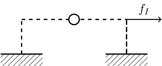
We summarize here basic concepts of structural dynamics which motivated the implementation of Namazu. For deeper insights and special cases, the interested reader is referred to [1][2]. An ideal linear system is submitted to a time-dependent ground motion \(x_g(t)\) as depicted in the figure below. The movement is such that the inertia effects cannot be neglected. All supports of the structure have the same displacement.

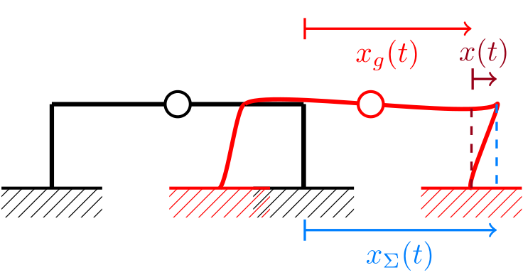
Idealized linear single-degree-of-freedom system of a frame structure under seismic ground motion \(x_g(t)\), [1].

Due to the ground’s movement, several reaction forces are occurring on the structure, Newton’s second law of motion states that a dynamic system is in equilibrium at each time instant. The occurring reaction forces are shown in the figure below. The displacement \(x(t)\) is in relation to the lateral resisting force \(F_L = kx(t)\), where \(k\) is the stiffness of the structure. Assuming damping is present, the damping force can be obtained by \(F_D = c \dot{x}(t)\), with \(c\) being the damping coefficient.

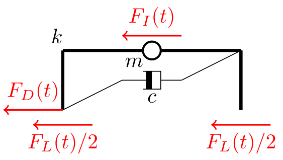
Free body system with reaction forces, dynamic equilibrium for each time instance \(t\).

The resulting total displacements of the structure are denoted by \(x_{\Sigma}(t)\). Since the ground motion is time-dependent, the following relation for the total displacement is given

\[x_{\Sigma}(t) = x_g(t) + x(t).\]

The inertia force \(F_I\) depends on the acceleration and mass of the structure, i.e. \(F_I = m \ddot{x}_{\Sigma}(t)\). The dynamic equilibrium gives

\[F_I(t) + F_D(t) + F_L(t) = 0.\]

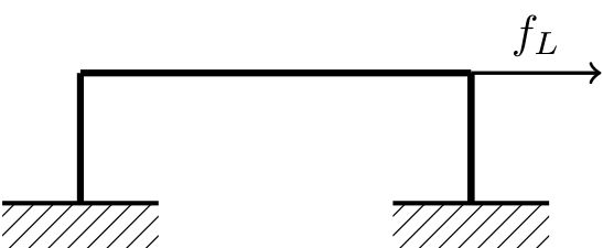
Lateral resisting force, connected to displacement \(x\). I mean the arrow direction is kinda unintuitive

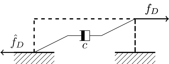
Damping force, connected to velocity \(\dot{x}\).

Inertia force related to mass components, connected to acceleration \(\ddot{x}_t\).

The equation of motion in a linear elastic case is thus given by

\[m\ddot{x}(t) + c\dot{x}(t) + k x(t) = -m \ddot{x}_g(t).\]

Hence the idea of a displacement-controlled experimental setup. The tunable shaking table should be able to model the seismic ground motion \(x_g(t)\) present, which is represented by the shaking table’s specimen plate movement. These motions can of course also be connected to other motions, such as the vibration of machinery, slides, or harmonic movements.

Signal Generation

Harmonic Signals

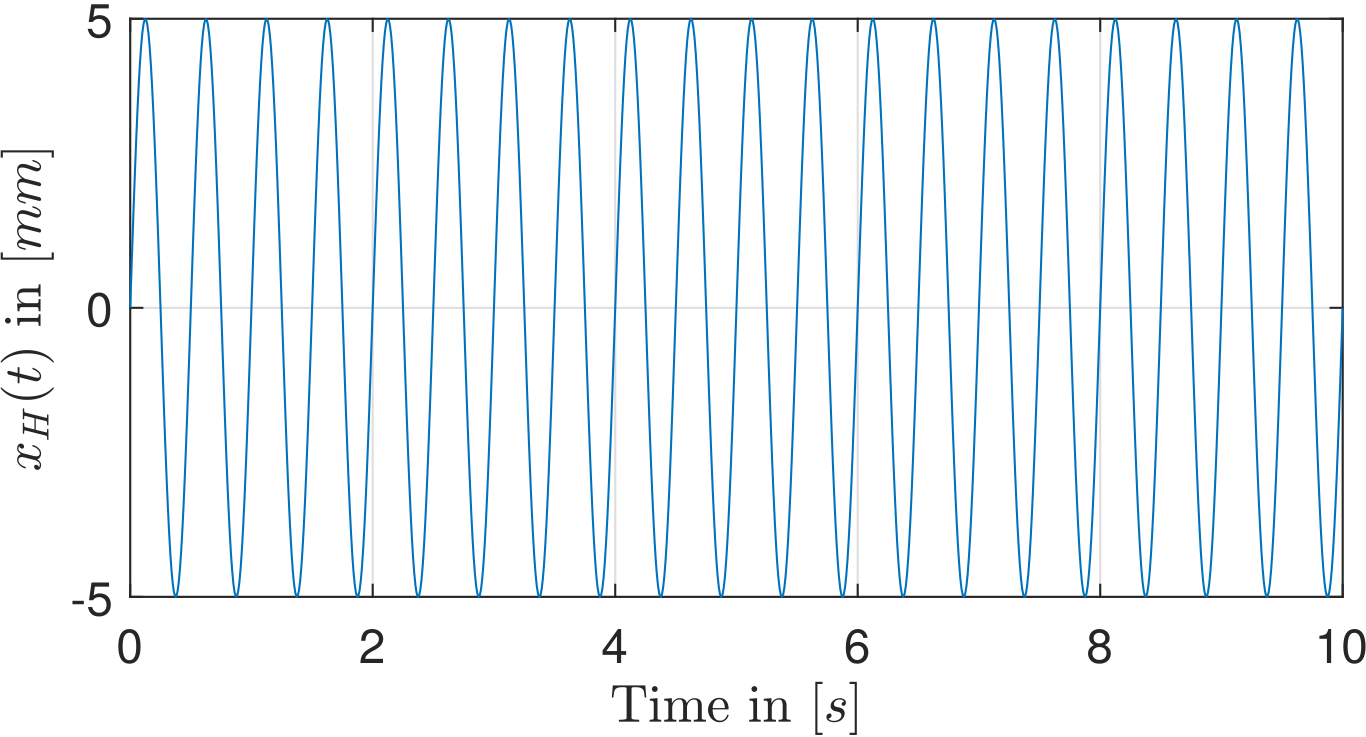
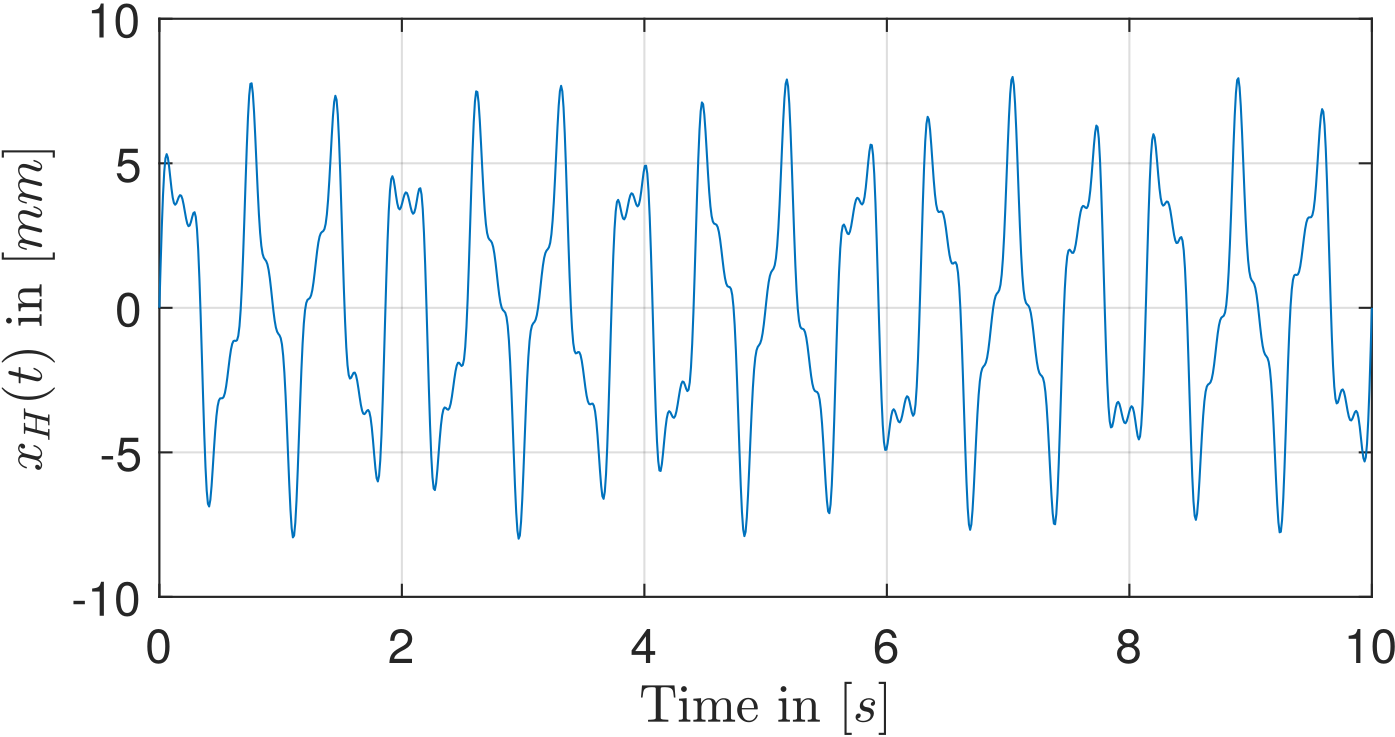
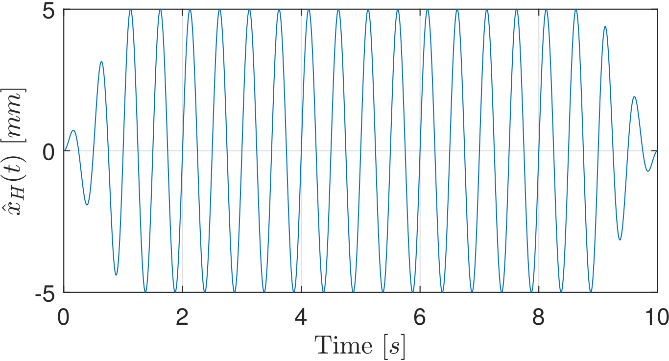
First, harmonic signals have been considered. They consist of a sum of frequency components and are closely related to the Fourier series. Choosing a number \(n_{\Omega}\) of frequencies, the position \(x_{H}(t)\) is calculated as the superposition of the harmonic frequencies and their respective amplitude factor by

(1)\[x_H(t) = \sum_{k=1}^{n_{\Omega}} \mathbb{A}_k \sin(2\pi\mathbf{\Omega}_kt),\]

where \(\mathbf{\Omega}_i \in \mathbb{R}_{\geq0}\) are the frequencies of interest and \(\mathbb{A}_i \in \mathbb{R}_{\geq0}\) the corresponding amplitude values with \(i \in [1, n_{\Omega}]\). The figures below show a fixed harmonic signal with a single frequency and a mixed harmonic signal with three superposed frequency components. These signals are deterministic.

Fixed harmonic signal with 2 Hz

Fixed harmonic signal with three overlapping frequencies

Stationary Stochastic Signals

Another class of signals of interest in structural engineering consists of uni-variate stationary Gaussian stochastic processes. They can be described by the Spectral Representation Method (SRM) from a functional frequency content, the so-called Power Spectral Density (PSD) function. The SRM and its variations, such as the Stochastic Harmonic Function (SHF) representation [3], are commonly used to simulate artificial ground motion [4][5].

Any PSD function can be used in the OpenVIBE framework according to the user preferences. Among possible PSD, the Shinozuka and Deodatis frequency content [6] referred to as the Shinozuka benchmark and defined by the following PSD

(2)\[ S_{S}(\omega) = \frac{1}{4} \sigma^2 b^3 \omega^2 e^{-b |\omega|},\quad -\infty < \omega < \infty,\]

is chosen. The constant \(\sigma\) corresponds to the standard deviation of the stochastic signal and \(b\) is a parameter that models the correlation distance of the stochastic signals [7]. The values \(\sigma = 1\) and \(b = 1\) are chosen. From the reference PSD, a realization of the stochastic signal denoted \(x_S(t)\) reads

(3)\[x_S(t) = \mathbb{A}_s \sum \limits_{n = 0}^{N-1} \sqrt{4 S_{x_{S}}(\omega_n) \Delta \omega} \cos(\omega_n t + \varphi_n).\]

The angular frequencies \(\omega_n\) in \(\text{rad/s}\) are defined as \(\omega_n = n \Delta \omega\) with \(n \in [0,N-1]\) and \(\Delta \omega = \omega_u/N\). The angular frequency \(\omega_u = 4\pi\ \text{rad/s}\) is the upper cut-off angular frequency, directly linked with the upper cut-off frequency as \(f_u = \omega_u /2\pi\) beyond which the PSD function vanishes. The corresponding time discretization is \(\Delta t = \pi/\omega_u\) in \([\text{s}]\) . The number of terms \(N\) is a choice which governs the accuracy of the approximation. The phase angles \(\varphi_n\) are independent realizations of a uniform distribution between \(0\) and \(2 \pi\) [6].

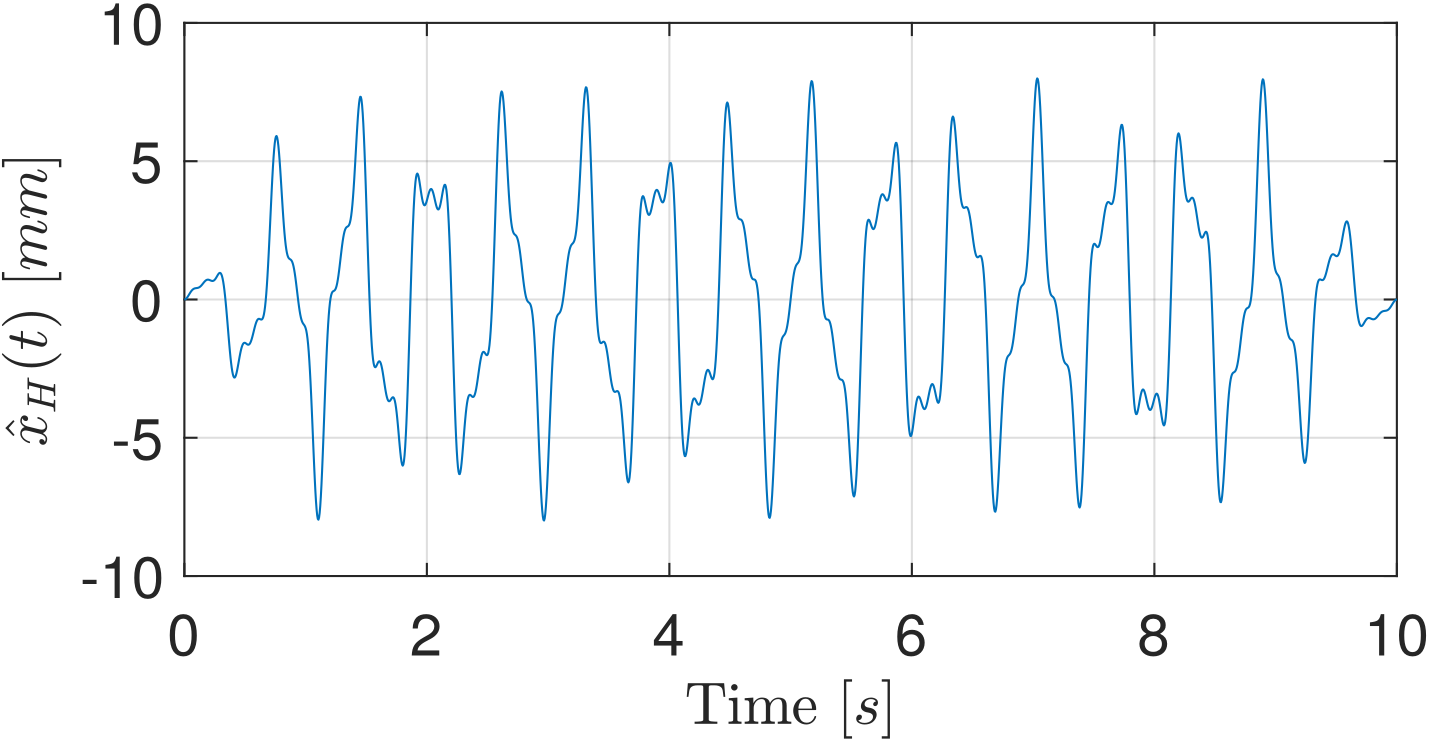
The signal magnitude is scaled by the factor \(\mathbb{A}_s \in \mathbb{R}_{\geq0}\) to achieve the displacement amplitude desired by the user. For instance, to reach a maximum displacement around \(17\ \text{mm}\), the scaling factor \(\mathbb{A}_s = 3\) has been chosen. One realization, i.e. a stochastic signal generated with the Shinozuka benchmark is shown here:

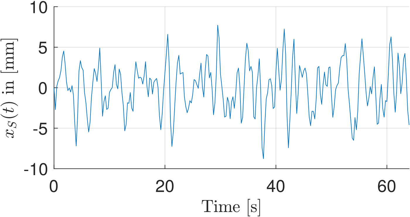
One realization of a random signal with the Shinozuka PSD (3) for \(N=128, \omega_u = 4\pi, \Delta t = \pi/\omega_u, T = 64 \text{s}, \mathbb{A}_s = 3\)

The periodogram [2][8][9] is used to estimate the signal PSD based on the discrete Fourier transformation of the random signals (3), as detailed in the Periodogram section. The direct approximation of the signal PSD by an estimator like the periodogram is usually not possible, as the target PSD is not known exactly for natural processes.

Shinozuka benchmark

We introduced the Shinozuka benchmark as a way of testing the frequency accuracy of the table and the framework. Usually, a single realization from a stochastic signal does not produce a nice looking PSD, but for certain input PSD functions this can be the case (e.g. (3)). While looking for ways to ensure that the framework does what it is supposed to do, the idea came up to use this property. Generating a signal from this PSD, then measuring the movement of the table and estimating the frequency contents with the Periodogram, we can easily assess divergences in the table’s behavior. The figure below shows the approximation of the Shinozuka PSD by the periodogram compared to the target PSD originally used to simulate the signal (2). All frequency components in the signal are preserved and thus the approximation is very accurate. The accuracy of the table can thus be evaluated by simulating one (or more for variance estimation) realizations with the Shinozuka PSD, measuring the displacement and then comparing the measured PSD to the original. For an accurate motion both PSDs should align. Therefore, the shaking table movement can be validated for the prescribed range of frequencies and accurate artificial ground motions of the shaking table will be expected for other stochastic signals generated by the SRM with similar frequency ranges to the Shinozuka benchmark.

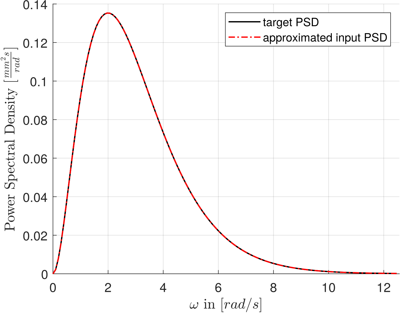
Shinozuka benchmark: scaled periodogram of one arbitrary realization (3) and target PSD (2)

Post-processing input signals for the shaking table

Some generated signals might require large initial accelerations or velocities due to the underlying numerical procedures. To circumvent these issues, we introduced post-processing procedures to ensure the safe usage of the shaking table.

First, for the harmonic signals \(x_H(t)\), artificial linear acceleration and deceleration phases based on a window-function are inserted. The acceleration phase lasts from \(t=0\) to \(t=t_u\) and the deceleration phase’s duration lasts from \(t=t_d\) to \(t = T\) such that the durations of acceleration and deceleration are \(t_u\) and \(T_d = T - t_d\), respectively. Then, the harmonic signal \(x_H(t)\) is adjusted from these two windows as

\[\begin{split}\hat{x}_H(t) = \begin{cases} \frac{t}{t_u} x_H, & t<t_u,\\ (1-\frac{t-T_d}{T-T_d}) x_H, &t>T_d,\\ x_H, &else. \end{cases}\end{split}\]

Considering \(t_u = t_d = 1\ \text{s}\), the harmonic signals from above are corrected to have adequate acceleration and deceleration:

Second, the position for the first time instance must always be zero, whereas it may not be a priori the case for the stochastic signal. This is achieved by zero padding for all signals, adding a zero position for the time instance \(t=0\). Only one time instant is added and not an acceleration ramp because the frequency content of the signal has to be preserved. It results in \(\hat{x}_S(t) = [0, x_S(t)]\) and the time discretization is adjusted to \(t \in [0,T+\Delta t]\):

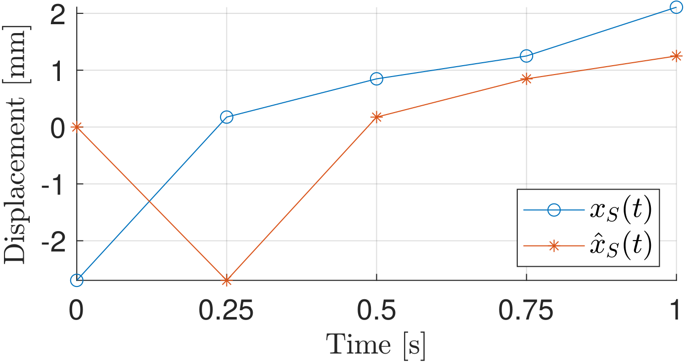
Comparison of an unmodified SRM signal \(x_S(t)\) and the zero-padded signal \(\hat{x}_S(t)\).

Other post-processing procedures, such as different window-functions for the ramp up and down are of course possible due to the open source nature of OpvenVIBE, but these are currently not implemented.

Periodogram

The periodogram [8] is an estimator to determine PSD functions from stochastic signals. It is defined as the squared absolute value of the discrete Fourier transform of a time signal \(X(t)\) as follows

(4)\[\hat{S}_X(\omega_k) = \lim \limits_{T \rightarrow \infty} \frac{\Delta t^2}{T} \left|\sum \limits_{t = 0}^{T-1} X(t) e^{-2 \pi i k t / T}\right|^2,\]

where \(T\) is the total number of discretized signal points and \(\Delta t\) the time increment. The time instant in the record \(t\) is just an index and \(k\) is the angular frequency discretization with \(\omega_k = \frac{2 \pi k}{T}\).

References

[1] (1,2)

A.K. Chopra. Dynamics of Structures. Pearson, Great Britain, 2007.

[2] (1,2)

Jie Li and Jianbing Chen. Stochastic Dynamics of Structures. John Wiley & Sons, Ltd (Asia), United States, 1 edition, 2010. URL: https://www.wiley.com/en-us/Stochastic+Dynamics+of+Structures-p-9780470824252.

[3]

Jianbing Chen, Fan Kong, and Yongbo Peng. A stochastic harmonic function representation for non-stationary stochastic processes. Mechanical Systems and Signal Processing, 96:31–44, 2017. URL: https://www.sciencedirect.com/science/article/pii/S0888327017301784, doi:https://doi.org/10.1016/j.ymssp.2017.03.048.

[4]

Meng-Ze Lyu, Jian-Bing Chen, and Jia-Xu Shen. Refined probabilistic response and seismic reliability evaluation of high-rise reinforced concrete structures via physically driven dimension-reduced probability density evolution equation. Acta Mechanica, pages 1619–6937, 2023. URL: https://www.sciencedirect.com/science/article/pii/S0267726122002858, doi:https://doi.org/10.1007/s00707-023-03666-4.

[5]

Shuoyu Liu, Liuliu Peng, Jun Liu, Shuang Zhao, and Zhongming Jiang. Spectral representation-based efficient simulation method for fully non-stationary spatially varying ground motions. Soil Dynamics and Earthquake Engineering, 161:107436, 2022. URL: https://www.sciencedirect.com/science/article/pii/S0267726122002858, doi:https://doi.org/10.1016/j.soildyn.2022.107436.

[6] (1,2)

Masanobu Shinozuka and George Deodatis. Simulation of stochastic processes by spectral representation. Applied Mechanics Reviews, 44(4):191–204, 1991. doi:10.1115/1.3119501.

[7]

M Shinozuka and G Deodatis. Response variability of stochastic finite element systems. Journal of Engineering Mechanics, 114(3):499–519, 1988.

[8] (1,2)

David Edward Newland. An introduction to random vibrations, spectral & wavelet analysis. Dover Publication, United States, 2012.

[9]

Marco Behrendt, Masaru Kitahara, Takeshi Kitahara, Liam Comerford, and Michael Beer. Data-driven reliability assessment of dynamic structures based on power spectrum classification. Engineering Structures, 268:114648, 2022. URL: https://www.sciencedirect.com/science/article/pii/S0141029622007453, doi:https://doi.org/10.1016/j.engstruct.2022.114648.